Transform Variography
The features described in this topic are only available if you have the Leapfrog Edge extension.
When data sets have highly skewed distributions, experimental variograms can be poorly structured and fitting a model can be difficult. Capping or discarding high values can help in certain situations but a better approach is to transform the data values into a more tractable distribution prior to calculating variograms. Transform variography offers a more general method that does not involve discarding or redefining data, reducing the effect that extreme values have on variogram calculations while retaining the ordering relationships between data values. Variogram models can be more easily defined and fitted in this transformed data space.
The transformed data cannot be used directly in estimations, however; transforming the data is solely for the purpose of fitting the variogram model. Having fitted the variogram model in transformed space, it is necessary to back-transform the variogram model before Kriging in the raw data space.
To transform data, start in the Values object in a domained estimation, and select Transform Values from the menu. This will add a new set of transformed values under the Values object in the project tree, with the same name as the original values but with NS (for Normal Score) appended. The transformation performed is a normal scores transformation, modifying the distribution of the data into a gaussian distribution. 30 polynomials are used to fit a Hermite polynomial model that describes the transformation between raw and gaussian values. Negative values are clamped at 0. As a result of the transform, the effects of outliers and clustered data is ameliorated. There is no independent declustering or despiking applied to the values during transformation. Drag the transformed values points into the scene to visualise them.
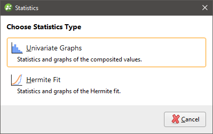
Statistics are available on the transformed values by right-clicking on them and selecting from the Choose Statistics Type options.
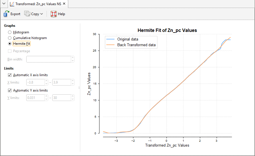
The standard Univariate Graphs option provides a histogram and other related plots of the transformed data. For more on univariate graphs, see Univariate Graphs. An option specific to transformed values, the Hermite Fit graph, has been added to show the fit of the Hermite polynomial to the cumulative distribution of the raw data.
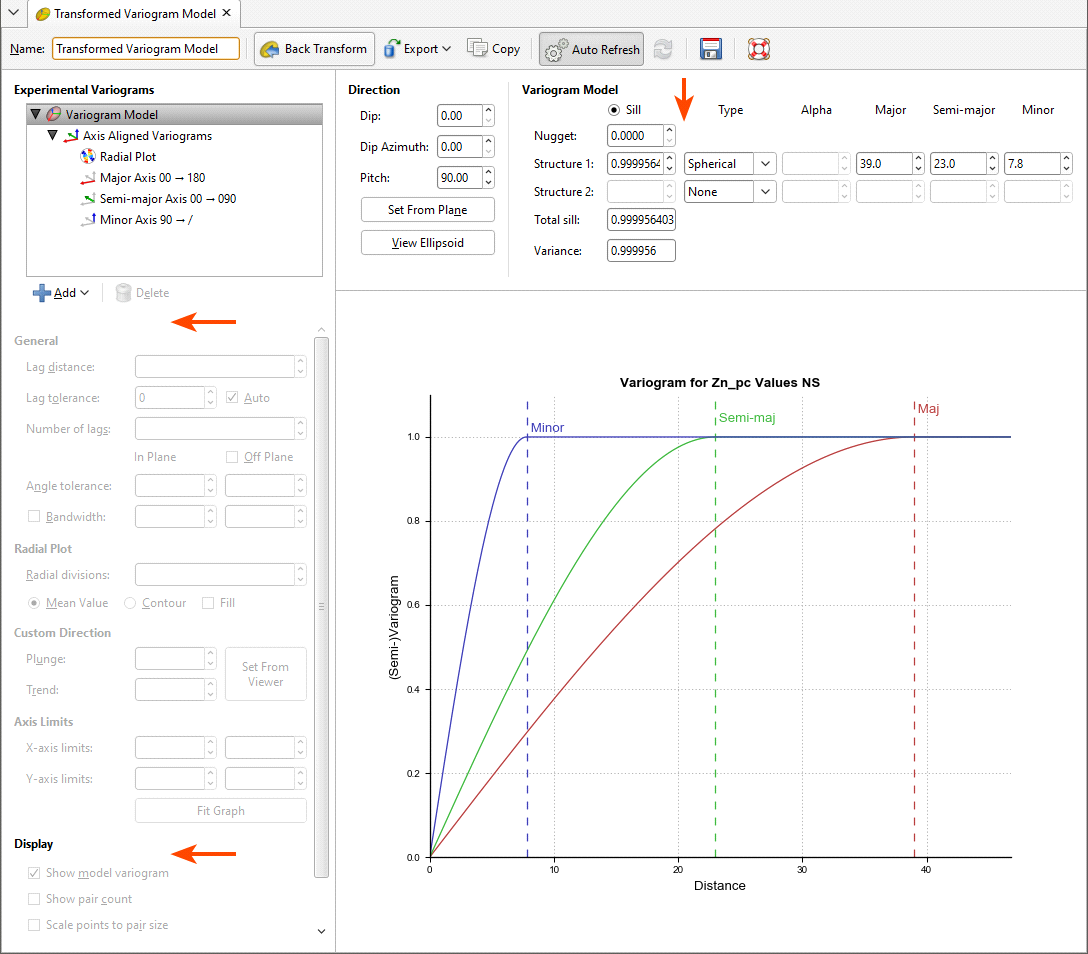
Create a New Transform Variogram Model by right-clicking on the Spatial Models folder and choosing the New Transformed Variogram Model option. You can then perform variography and fit a variogram model as you would for a typical variogram model. There is no automated fitting, just as for the typical variogram. Note that capping has been removed, there is no normalised sill option, and variogram displays other than the semi-variogram are unavailable.
Once the model has been fitted to the transform variogram, click the Back Transform button. This will convert the variogram back into the untransformed raw data space.
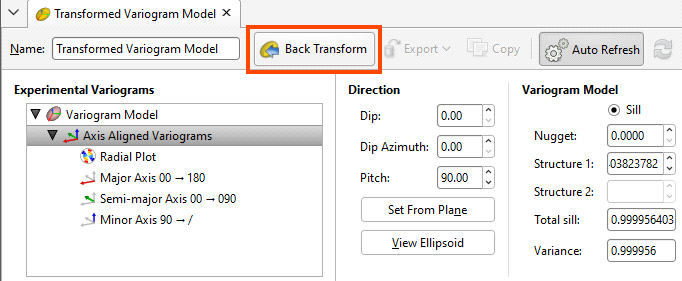
Once back-transformed, the variogram model cannot be manipulated with handles or directly into fields. A summary of the variogram parameters and orientation is provided in fixed text fields at the top of the window. Experimental controls are removed and only the display options remain.
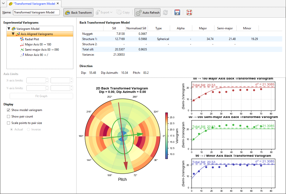
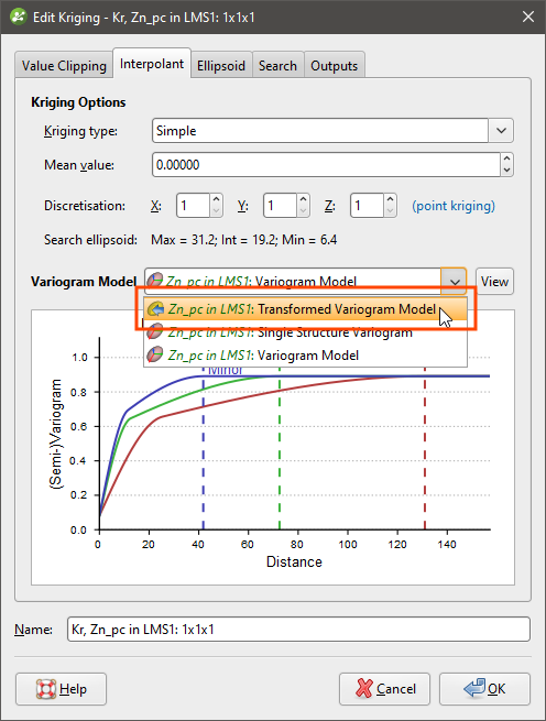
The transformed variogram model is not available for use in Kriging as the relative nugget and sills of the model in transformed space are generally considered optimistic. Once the model is back-transformed into the raw data space, the back transformed variogram model can be selected for use in Kriging, just like any of the untransformed models.
Got a question? Visit the Seequent forums or Seequent support