Standard Estimators

Leapfrog Geo supports the following estimator functions:

• Inverse distance
• Nearest neighbour
• Ordinary and simple Kriging
• RBF (Radial Basis Function)

This topic describes creating and working with the different types of estimators. It is divided into:

• Inverse Distance Estimators
• Nearest Neighbour Estimators
• Kriging Estimators
• RBF Estimators
• Sample Geometries
• Combined Estimators

Estimators can be copied, which makes it easy to experiment with different parameters. Simply right-click on the estimator in the project tree and select Copy.

Inverse Distance Estimators

The basic inverse distance estimator makes an estimate by an average of nearby samples weighted by their distance to the estimation point. The further a data point is from the estimate location, the less it will be relevant to the estimate and a lower weight is used when calculating the weighted mean.

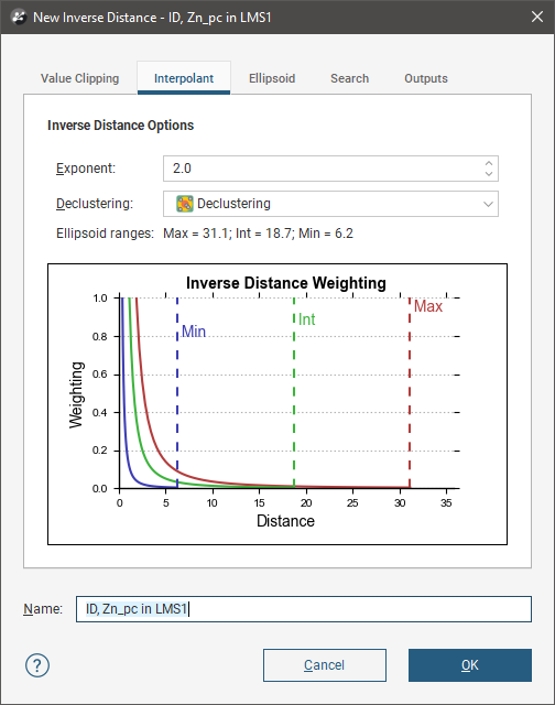
To create an inverse distance estimator, right-click on the Estimators folder and select New Inverse Distance Estimator. The New Inverse Distance window will appear:

Leapfrog Geo extends the basic inverse distance function, and the inverse distance estimator supports declustering and anisotropic distance.

In the Interpolant tab:

• Exponent adjusts the strength of the weighting as distance increases. A higher exponent will result in a weaker weight for the same distance.
• Optionally select a Declustering object from the declustering objects defined for the domained estimation; these are saved in the Sample Geometry folder.
• Ellipsoid Ranges identify the Max, Int and Min ranges set in the Ellipsoid tab.
• A chart depicts the resultant weights that will be applied by distance.

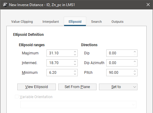
In the Ellipsoid tab:

• The Ellipsoid Definition sets the anisotropic distance and direction, scaling distances in three orthogonal directions proportionally to the range for each of the directions of the ellipsoid axes. This effectively makes the points in the direction of greater anisotropy appear closer and increases their weighting. Adjust the Ellipsoid Ranges and Directions to describe the anisotropic trend.
• Click View Ellipsoid to see an ellipsoid widget in the scene that helps to visualise the anisotropic trend.

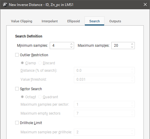
In the Search tab:

• The Minimum Samples and Maximum Samples parameters determine the number of samples required or used within the search neighbourhood.
• The remaining fields provide controls to reduce bias.
  • Outlier Restriction reduces bias by constraining the effect of high values at a distance. After ticking Outlier Restriction, you can choose to either Clamp (reduce the high value to the Value Threshold) or Discard high values that meet the criteria for outlier restrictions. It limits the samples that will be considered to those within a specified Distance percentage of the search ellipsoid size, and only those outside that distance if they are within the Value Threshold. If a sample point is beyond the Distance threshold and the point's value exceeds the Value Threshold, it will be clamped or discarded according to the option selected.
  • Sector Search divides the search space into sectors. Choose from Octant providing eight sectors or Quadrant providing four sectors. The Maximum samples per sector threshold specifies the number of samples in a sector before more distant samples are ignored. The Maximum empty sectors threshold specifies how many sectors can have no samples before the estimator result will be set to the non-normal value without_value.
  • Drillhole Limit constrains how many samples from the same drillhole will be used in the search before limiting the search to the closest samples in the drillhole and looking for samples from other drillholes.

In the Value Clipping tab, you can enable value clipping by ticking the Clip input values box. This caps values outside of the range set by the Lower bound and Upper bound to the bounding values.

In the Outputs tab, you can specify attributes that will be calculated when the estimator is evaluated on a block model. Value and Status attributes will always be calculated, but you can choose additional attributes that are useful to you when validating the output and reporting. These attributes are:

• The number of samples (NS) is the number of samples in the search space neighbourhood.
• The distance to the closest sample (MinD) is a cartesian (isotropic) distance rather than the ellipsoid distance.
• The average distance to sample (AvgD) is the average distance using cartesian (isotropic) distances rather than ellipsoid distances.

• The number of duplicates deleted (ND) indicates how many duplicate sample values were detected and deleted by the estimator.
• When the estimator must select from equidistant points to include or exclude in the search space because it found more samples than the Maximum Samples threshold, the number of equidistant points detected (EquiD) is recorded. You can use this output as a trigger for further investigation.

Nearest Neighbour Estimators

Nearest neighbour produces an estimate for each point by using the nearest value as a proxy for the location being estimated. There is a higher probability that the estimate for a location will be the same as the closest measured data point, than it will be for some more distance measured data point.

To create a nearest neighbour estimator, right-click on the Estimators folder and select New Nearest Neighbour Estimator. The New Nearest Neighbour window will appear:

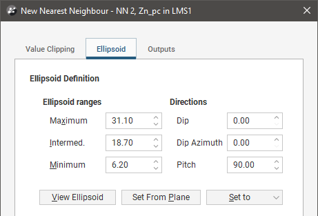
Nearest Neighbour uses an astral search algorithm to determine what point is considered the nearest. Leapfrog Geo includes support for anisotropy when determining what is considered the ‘nearest’ value. Adjust the Ellipsoid Ranges and Directions to describe the anisotropic trend.

Click View Ellipsoid to see an ellipsoid widget in the scene that helps to visualise the anisotropic trend.

In the Value Clipping tab, you can enable value clipping by ticking the Clip input values box. This caps values outside of the range set by the Lower bound and Upper bound to the bounding values.

In the Outputs tab, you can specify attributes that will be calculated when the estimator is evaluated on a block model. Value and Status attributes will always be calculated, but you can choose additional attributes that are useful to you when validating the output and reporting. These attributes are:

• The number of samples (NS) is the number of samples in the search space neighbourhood.
• The distance to the closest sample (MinD) is a cartesian (isotropic) distance rather than the ellipsoid distance.
• The average distance to sample (AvgD) is the average distance using cartesian (isotropic) distances rather than ellipsoid distances.

Kriging Estimators

Kriging is a well-accepted method of interpolating estimates for unknown points between measured data. Instead of the simplistic inverse distance and nearest neighbour estimates, covariances and a Gaussian process are used to produce the prediction.

To create a Kriging estimator, right-click on the Estimators folder and select New Kriging Estimator. The New Kriging window will appear:

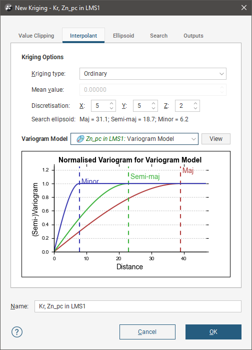
In the Interpolant tab:

• Both Ordinary and Simple Kriging are supported.
• For Simple Kriging, specify a Mean value for the local mean to use in the Kriging function.
• Discretisation sets the number of discretisation points in the X, Y and Z directions for block Kriging. Block Kriging provides a means of estimating the best value for a block instead of only at the centre of the block. Each block is broken down (discretised) into a number of sub-units without actually sub-blocking the blocks. A geologist will consider a variety of factors including spatial continuity when deciding on the discretisation to use. Set the X, Y and Z parameters to 1 for point Kriging. To use additional discretisations, copy the estimator and change the Discretisation parameters.
• Search Ellipsoid identifies the Max, Int and Min ranges set in the Ellipsoid tab.
• Select from the Variogram Model list of models defined in the Spatial Models folder.
• The View button will show an ellipsoid widget in the scene to assist in visualising the variogram model ranges and direction.
• A chart depicts colour-coded semi-variograms for the variogram model.

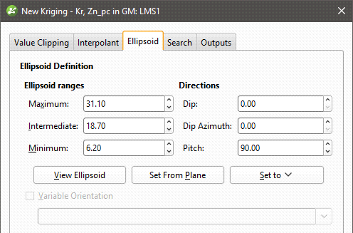
In the Ellipsoid tab:

• The Ellipsoid Definition sets the Ellipsoid Ranges and Direction.
• Click the View Ellipsoid definition to show an ellipsoid widget in the scene to assist in visualising the search ellipsoid. Note that this is not the same as the variogram model ellipsoid, unless the Set to option is used to select the variogram model to copy the details.

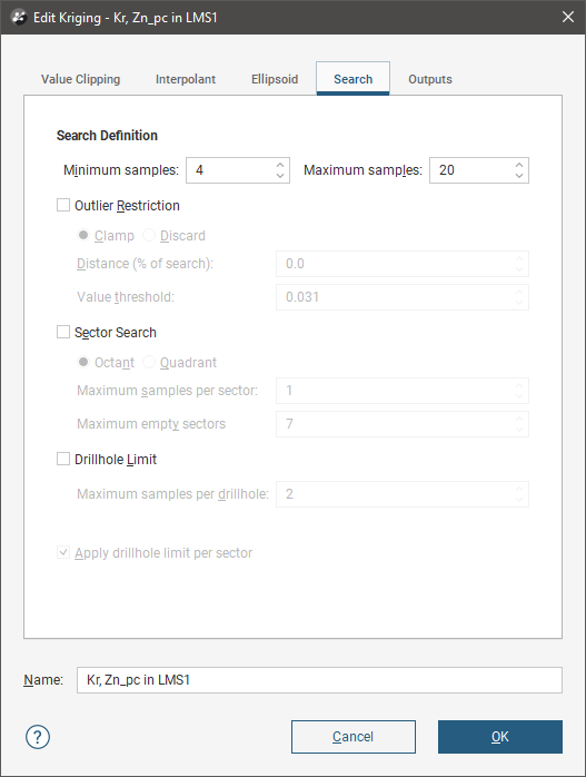
In the Search tab:

• The Minimum Samples and Maximum Samples parameters determine the number of samples required or used within the search neighbourhood.
• The remaining fields provide controls to reduce bias.
  • Outlier Restriction reduces bias by constraining the effect of high values at a distance. After ticking Outlier Restriction, you can choose to either Clamp (reduce the high value to the Value Threshold) or Discard high values that meet the criteria for outlier restrictions. It limits the samples that will be considered to those within a specified Distance percentage of the search ellipsoid size, and only those outside that distance if they are within the Value Threshold. If a sample point is beyond the Distance threshold and the point's value exceeds the Value Threshold, it will be clamped or discarded according to the option selected.
  • Sector Search divides the search space into sectors. Choose from Octant providing eight sectors or Quadrant providing four sectors. The Maximum samples per sector threshold specifies the number of samples in a sector before more distant samples are ignored. The Maximum empty sectors threshold specifies how many sectors can have no samples before the estimator result will be set to the non-normal value without_value. When Sector Search is enabled, the translucent planes in the search ellipsoid widget change to show the search sectors.
  • Drillhole Limit constrains how many samples from the same drillhole will be used in the search before limiting the search to the closest samples in the drillhole and looking for samples from other drillholes.

  • The Apply drillhole limit per sector option controls the behaviour of the application of the sector search and drillhole limits. It is only available when both Sector Search and Drillhole Limit settings are being used. When the box is ticked, the Drillhole Limit setting for Maximum samples per drillhole is applied per sector, so a drillhole may have more samples per drillhole than is specified in the limit, but the number is constrained to the limit for each sector the drillhole passes through. When unticked, the Drillhole Limit setting for Maximum samples per drillhole is applied without regard to which sectors the drillhole passes through, and this may reduce the number of samples available for the search.

In the Value Clipping tab, you can enable value clipping by ticking the Clip input values box. This caps values outside of the range set by the Lower bound and Upper bound to the bounding values.

Kriging Attributes

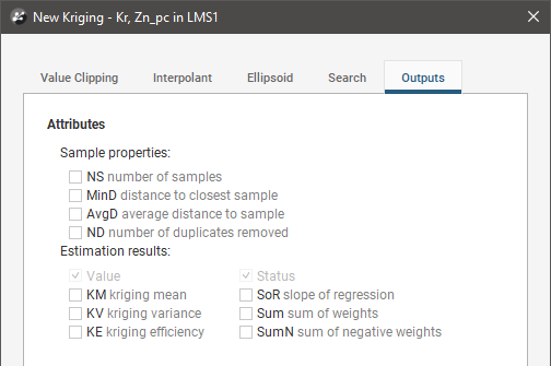
In the Outputs tab, you can specify attributes that will be calculated when the estimator is evaluated on a block model. Value and Status attributes will always be calculated, but you can choose additional attributes that are useful to you when validating the output and reporting. These attributes are organised into two categories, Sample properties and Estimation results.

Sample properties are output attributes that relate to data sample statistics:

• The number of samples (NS) is the number of samples in the search space neighbourhood.
• The distance to the closest sample (MinD) is a cartesian (isotropic) distance rather than the ellipsoid distance.
• The average distance to sample (AvgD) is the average distance using cartesian (isotropic) distances rather than ellipsoid distances.
• The number of duplicates deleted (ND) indicates how many duplicate sample values were detected and deleted by the estimator.

Estimation results are additional information produced by the estimation:

• Value will always be included as it is the actual estimate result.
• Status will always be included as it classifies the estimation result as a Normal result, or non-normal Blank, Without-value, Outside or Error result.
• The Kriging mean (KM) is the local mean used for the estimate based around the selected sample data. For simple Kriging, this is the specified global mean. For ordinary Kriging, it is the unknown locally constant mean that is assumed when forming the Kriging equations. This value is only dependent on the covariance function and the sample locations and values for the chosen neighbourhood. It does not depend on the evaluation volume and therefore will be the same for block Kriging and point Kriging. It can give some indication of suitability of the assumptions when doing ordinary Kriging.
• The Kriging variance (KV) is important in assessing the quality of an estimate. It grows when the covariance between the samples and the point to estimate decreases. This means that when the samples are further away from the evaluation point, the quality of the estimation decreases. For simple Kriging, the value is capped by the value of the covariance between the target volume and itself. For ordinary Kriging, higher values indicate a poor value.
• The Kriging efficiency (KE) is calculated based on the block variance and Kriging variance (KV). It should be 1 when the Kriging variance is at is minimum and 0 when the Kriging variance equals the block variance.
• The slope of regression (SoR) is the slope of a linear regression of the actual value, knowing the estimated value. For simple Kriging it is 1 and for ordinary Kriging a value of 1 is desired as it indicates that the resulting estimate is conditionally unbiased. Conditional bias is to be avoided as it increases the chance that blocks will be misclassified when considering a cutoff value.
• The sum of weights (Sum) is the sum of the Kriging weights. For ordinary Kriging, the sum is constrained to being equal to 1.
• The sum of negative weights (SumN) can be used to assess the quality of an estimation. Negative weights are to be avoided or at least minimised. If there are negative weights, it is possible that the estimated value may be outside the range of the sample values. If the sum of negative weights is significantly large (when compared to the total sum), then it could result in a poorly estimated value, depending on the sample values.

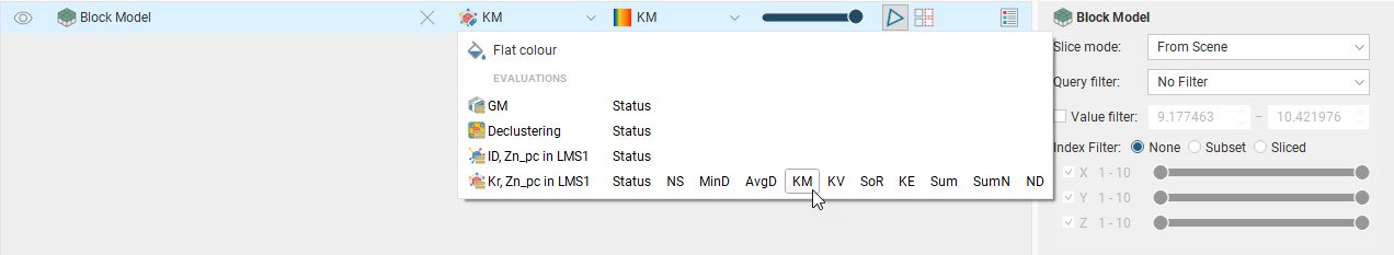
When selecting the block model evaluation to display in the 3D scene, you can select either the Kriging values, or from these additional selected attributes.

RBF Estimators

The RBF estimator brings the Radial Basis Function used elsewhere in Leapfrog into estimation. Like Kriging, RBF does not use an overly-simplified method for estimating unknown points, but produces a function that models the known data and can provide an estimate for any unknown point. Where Kriging is limited to a local search neighbourhood, RBF utilises a global neighbourhood. An RBF estimator is good for grade control where there is a large amount of data.

To create an RBF estimator, right-click on the Estimators folder and select New RBF Estimator. The New RBF window will appear:

Like other estimators, a spatial model defined outside the estimator as a separate Variogram Model can be selected. The View button will show an ellipsoid widget in the scene to assist in visualising the variogram model ranges and direction.

Alternatively, in a feature unique to RBF estimators, a Structural trend can be used, if one is available in the project. Set the Outside value at the long-range mean value of the data.

Otherwise, the RBF estimator behaves very similarly to the RBF interpolant in Leapfrog.

Drift is used to specify what the estimates should trend toward as distance increases away from data. The RBF estimator has different Drift options from the non-estimation RBF interpolants. The RBF estimator function offers the Drift options Specified and Automatic. When selecting Specified, provide a Mean Value for the trend away from data. Automatic is equivalent to the Constant option offered by non-estimation RBF interpolants, and Linear is not supported. Specified drift with a Mean Value of 0 is equivalent to None.

In the Value Clipping tab, you can enable value clipping by ticking the Clip input values box. This caps values outside of the range set by the Lower bound and Upper bound to the bounding values.

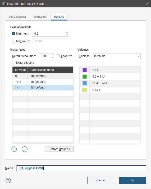
In the Outputs tab, the Minimum and MaximumEvaluation Limits constrain the values. Values outside the limits are set to either the minimum or maximum limit, as appropriate. To enable a limit, tick the checkbox and set a limit value.

In the Outputs tab, you can also define isosurfaces for an RBF estimator:

• The Default resolution will be used for all isosurfaces, unless you change the Surface Resolution setting for an individual isosurface. See Surface Resolution in Leapfrog Geo for more information on the Adaptive setting. The resolution can be changed once the estimator has been created, so setting a value in the New RBF window is not vital. A lower value will produce more detail, but calculations will take longer.
• The Volumes enclose option determines whether the volumes enclose Higher Values, Lower Values or Intervals. Again, this option can be changed once the estimator has been created.
• Click the Restore Defaults button to add a set of isosurfaces based on the estimator’s input data.
• Use the Add to add a new isosurface, then set its Iso Value.
• Click on a surface and then on the Remove button to delete any surface you do not wish to generate.

Sample Geometries

The declustering object is a tool for calculating local sample density. It can be used to provide confidence in an estimate, a value for determining boundaries, or a declustering weight that can be used to remove sampling bias from a set of values. Common traditional techniques for declustering utilise a grid or polygonal cells.

In Leapfrog Geo, the declustering object is used to calculate declustering weights that are inversely proportional to the data density at each sample point. A declustering object can be used by an inverse distance estimator.

Creating a New Declustering Object

To create a new declustering object, right-click on the Sample Geometry folder and select New Declustering Object. The New Declustering Object window will appear and an ellipsoid will be added to the scene.

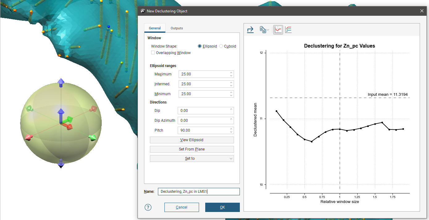
The ellipsoid assists in visualising the declustering window dimensions and direction. It is used for both the EllipsoidWindow Shape and the CuboidWindow Shape. For more information on how to work with the ellipsoid, see The Ellipsoid Widget. If the ellipsoid is removed from the scene it may be restored by clicking the View Ellipsoid button.

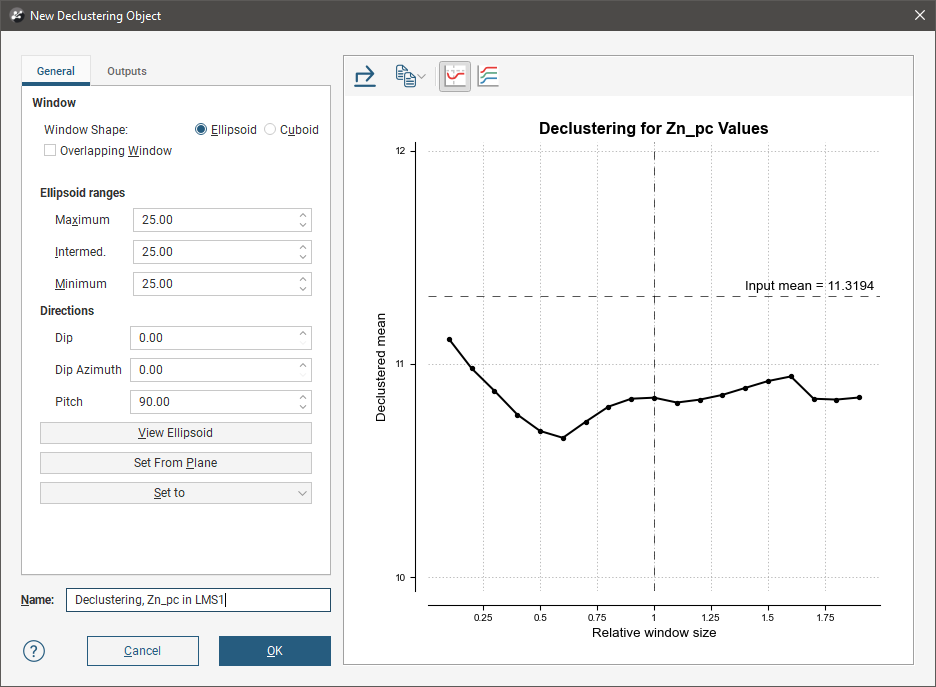
On the right side of the New Declustering Object window is a declustering chart. This is used to guide the selection of settings for the declustering object, particularly the ranges for the search ellipsoid. There are two chart views. The default ratio view, with the Ratio button () selected, shows a chart of the declustered mean against relative window size:

The range view, with the Range button () selected, shows three declustering charts, one for each axis of the search ellipsoid:

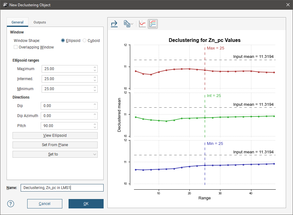
All charts indicate the naïve mean using a dotted horizontal line.

You can interact with the charts by dragging the dotted vertical line to the left or right. In the ratio view, this changes the current ellipsoid range settings by a proportional ratio, as indicated on the x-axis of the chart. In the range view, the selected range setting is updated accordingly. Select a place on the chart that minimises the effect of declustering on the mean of the data, where the range is close to the naïve mean and where there is no significant jump in the data.

Changes made to the declustering options are reflected automatically in the selected chart.

Above the chart are some export options. The Export button () saves the declustering chart as either a PDF, SVG or PNG file based on your selection. The Copy button () opens a menu with the option to Copy Graph Image to save an image to the operating system clipboard at the selected resolution. The three resolution options also appear in this menu. You can then paste the image into another application.

General Settings

The General tab of the New Declustering Object window is divided into three parts, Window, Ellipsoid Ranges and Directions.

The Window section defines the declustering object’s shape:

• The Window Shape can be Ellipsoid or Cuboid. Select Cuboid to approximate traditional grid declustering. The Ellipsoid option avoids increased density values for sampling oriented away from axes.
• The Overlapping Window option acts similarly to a rolling average by moving the window incrementally in overlapping steps, providing a much smoother result.
  • Disabling Overlapping Window approximates a traditional grid behaviour; a single fixed window is used around each evaluation location and the density is simply the count of all input points within the window.
  • Enabling Overlapping Window implicitly averages the point count over all possible windows that contain the evaluation location.

The Ellipsoid Ranges settings provide the same anisotropy controls used elsewhere in Leapfrog Geo, determining the relative shape and strength of the ellipsoid in the scene. Including them here provides additional advantages over traditional grid declustering.

• The Maximum value is the range in the direction of the major axis of the ellipsoid.
• The Intermediate value is the range in the direction of the semi-major axis of the ellipsoid.
• The Minimum value is the range in the direction of the minor axis of the ellipsoid.

The Directions settings determine the orientation of the ellipsoid in the scene, where:

• Dip and Dip Azimuth set the orientation of the plane for the major and semi-major axes of the ellipsoid. Dip is the angle off the horizontal of the plane, and Dip Azimuth is the compass direction of the dip.
• Pitch is the angle of the ellipsoid’s major axis on the plane defined by the Dip and Dip Azimuth. When Pitch is 0, the major axis is perpendicular to the Dip Azimuth. As Pitch increases, the major axis points further down the plane towards the Dip Azimuth.

The moving plane can also be useful in setting the anisotropy Directions. Add the moving plane to the scene, and adjust it using its controls. Then click the Set From Plane button to populate the Dip, Dip Azimuth and Pitch settings.

You can also use the Set to list to choose different from the variogram models available in the project.

Outputs

The Outputs tab of the New Declustering Object window features Attributes to calculate. Value and Status will always be calculated, but you can optionally include NS (number of samples), MinD (distance to closest sample) or AvgD (average distance to sample).

The Declustering Object in the Project Tree

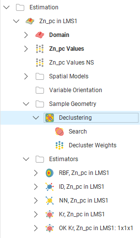
Enter a name for the declustering object and click OK to create it. It will be added to the project tree in the Sample Geometry folder. Expand it to see its parts, which can be individually added to the scene:

Double-click on the declustering object in the tree to edit it.

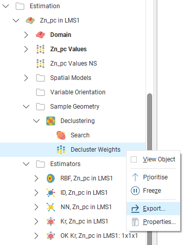
Export the declustering weights by right-clicking on the values object in the project tree and selecting Export.

Applying a Declustering Object

Leapfrog Geo supports declustering in the inverse distance estimator. To decluster data, select a declustering object from the Declustering dropdown list:

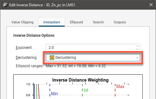
When no declustering object is selected, the inverse distance estimator is the standard inverse distance weighted method.

Combined Estimators

Combined estimators evaluates more than one estimation at a time on a block model. You can get a block model displaying a combined estimator showing more than one domained estimation result column or attribute.

Practical uses for this:

• To allow multiple estimation passes over the same domain, with more relaxed search criteria for subsequent passes.
• To estimate for different domains, either separate or overlapping, and evaluate them on the same block model.

By placing the estimations in a hierarchy, a preference can be indicated where different estimates are produced for the same block. Estimations lower in the hierarchy will be used when the higher-priority estimate results in a Without-value or Outside result.

Combined estimator work with Kriging, Nearest Neighbour, and Inverse Distance estimators. It does not work with RBF estimators. Generation of extended Kriging attributes is possible, but only when all the estimators in a combined estimator are Kriging estimators.

Creating a Combined Estimator

To create a combined estimator, right-click on the Estimation folder and select New Combined Estimator. The New Combined Estimator window will be displayed:

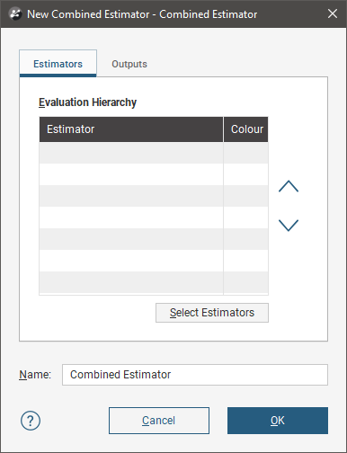
This window is divided into two tabs:

• Estimators
• Outputs

Adding Estimators to a Combined Estimator

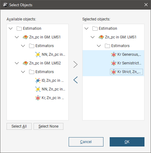
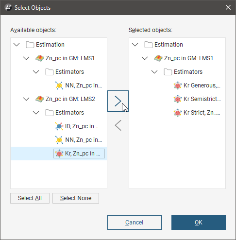
Click the Select Estimators button below the Evaluation Hierarchy. In the Select Objects window, choose from the Available objects the estimators you want to be in the combined estimator and click the right-arrow button to move them into the Selected objects list. Click OK to return to the New Combined Estimator window.

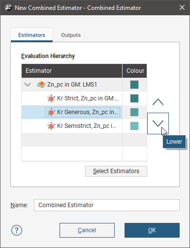
Reorder the estimators in the hierarchy by selected an estimator and clicking the Up ()or Down () buttons to move it up or down the list.

Give the combined estimator a recognisable identifying label by changing the Name.

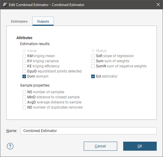
In the Outputs tab, select attributes you wish to be generated along with the estimate.

Value and Status will always be generated. Other attributes may be selected if all the estimators are Kriging estimators. If one or more estimators is a nearest neighbour or inverse distance estimator, many of the attributes will not be available.

Most of the attributes are identical to those described for the Kriging estimator. See Kriging Attributes for more information.

Two attributes specific to combined estimators are new category/lithology columns:

• Dom (domain), which domain from the domained estimations the evaluation came from.
• Est (estimator), which estimator was used to estimate the block.

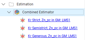
When you click OK a new combined estimator will appear in the Estimation folder. Below it will be links to the estimators that are being combined.

Evaluating a Combined Estimator

Combined estimators can only be evaluated on a block model. Right click a block model and select Evaluations, then select a combined estimator from the Available evaluations and add it to the Selected evaluations list. Click OK.

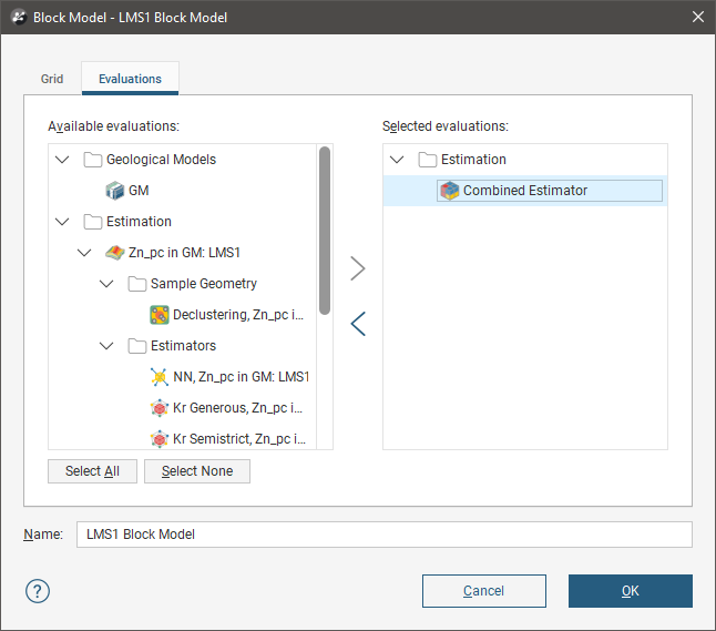
The block model with the evaluated combined estimator can be added to the scene.

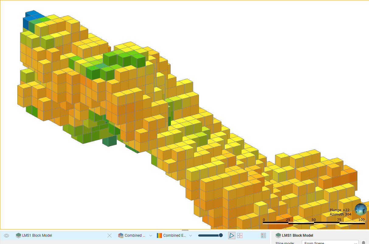
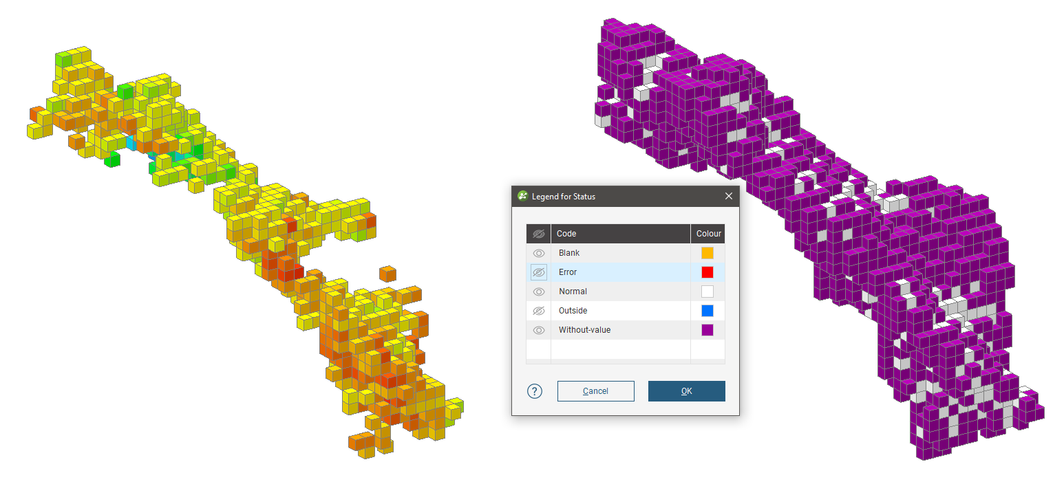
In this example, three estimators use progressively more generous search space and limits. The most strict estimator produces high confidence estimates, but over a small subset of the blocks in the block model. The block model is shown with two views; one displaying the estimate values, the other showing status, and specifically the Normal and Without-value blocks.

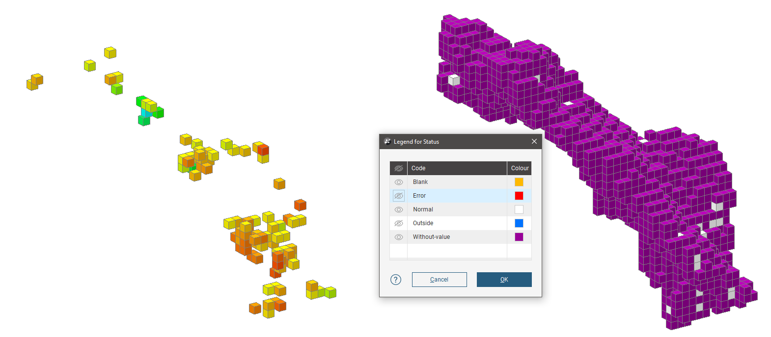
A larger search space produces estimates for more blocks, but many are still Without-value.

A much larger search space and reduced limits produces results for almost all the blocks in the domain.

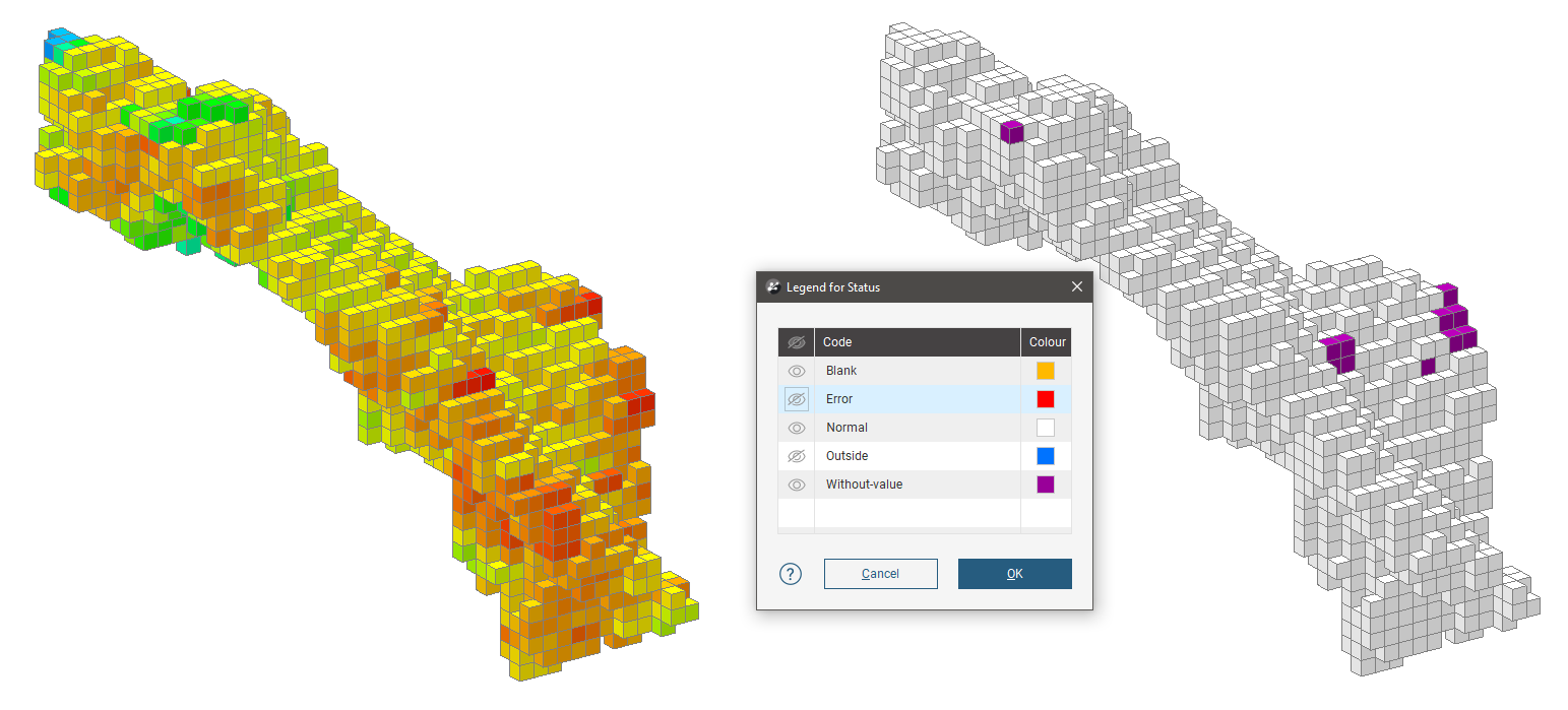
When these estimates are combined in that order, the blocks are only represented by an estimate if it has not already been given an estimate by a higher priority estimate in the hierarchy. The resulting block model evaluation may look a lot like the estimate with the most blocks, but an inspection of the evaluations of each of the blocks would reveal the subtle differences where blocks have been estimated with higher priority estimators.

Alternatively, you may have two different, possibly overlapping domain meshes. You can evaluate each domained estimation on a block model one at a time, but not in the same scene.

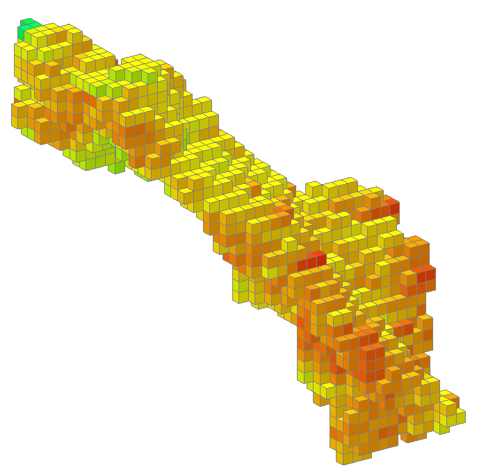
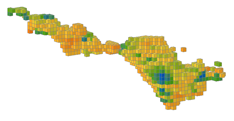
Using combined estimators we can combine the estimator used for this block model:

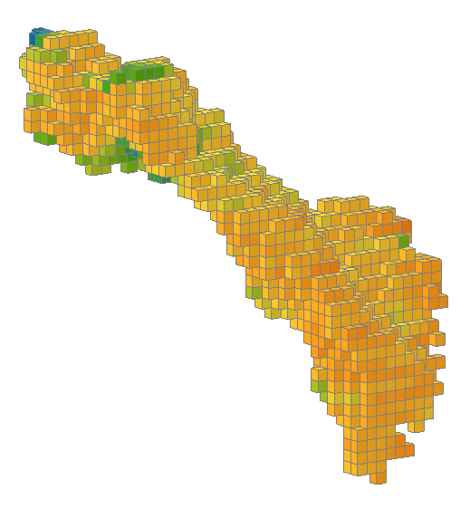
...with the estimator used for this block model.

Right click the Estimations folder and select New Combined Estimator. Click the Select Estimators button. Add an estimator from the domained estimations for each of these separate (and possibly overlapping) domains to the Selected objects.

When you click OK, the New Combined Estimator window shows the selected estimators within their domained estimations.

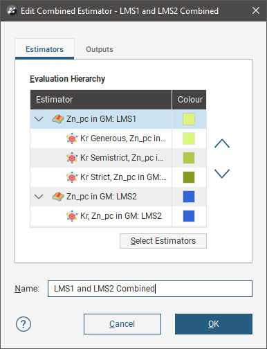
You can click the colour chip next to the domained estimation to choose an alternate base colour for the domained estimation. The colours for each of the estimators within a domained estimation are selected automatically as variations on the base colour, and cannot be customised.

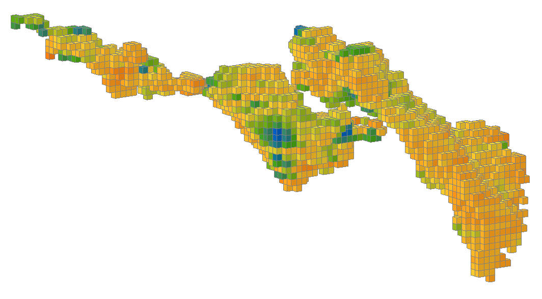
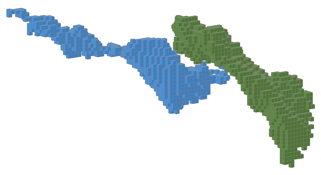
When the combined estimator is evaluated onto a block model, all the estimated blocks can be displayed in the scene, combining the domains.

Instead of displaying the estimated values, the Dom (domain) attribute may be shown instead, clearly indicating which blocks in the scene are in which domain.

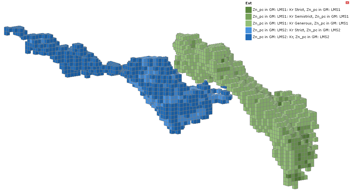
Here more estimators have been added to the combined estimator.

When displaying the Est (estimator) attributes, the colour variation from the base domain colour shows the different estimators used to evaluate the blocks.

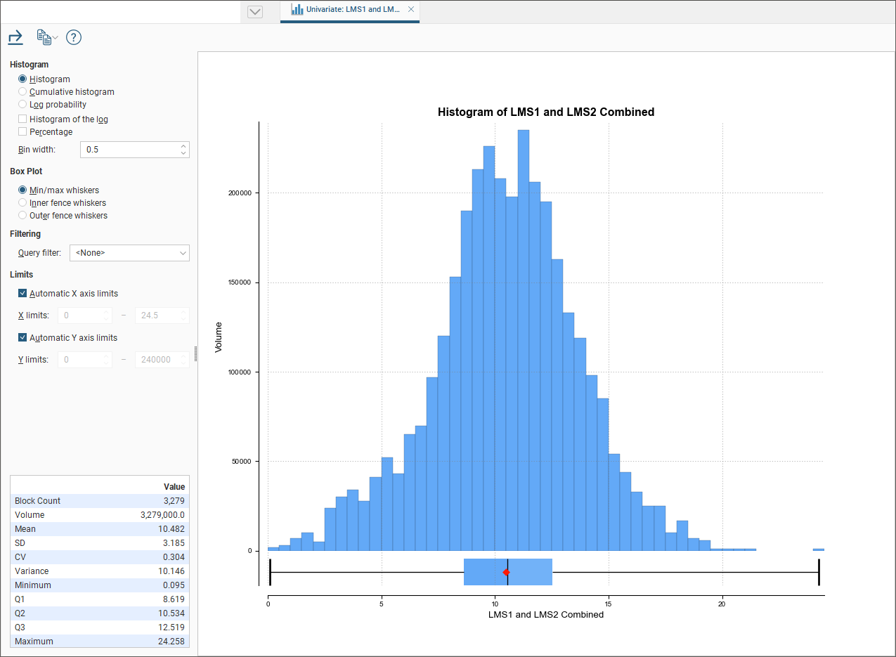
Viewing Statistics

Right click a combined estimator evaluation on a block model, and select Statistics. For more information on the univariate statistics displayed, see Univariate Graphs.

Copying a Combined Estimator

Right click a combined estimator in the Estimation folder and select Copy. You will be given an opportunity too choose a new name for the copy, and then it will appear in the project tree in the Estimation folder.

 

Got a question? Visit the Seequent forums or Seequent support