Variable Orientations
The features described in this topic are only available if you have the Leapfrog Edge extension.
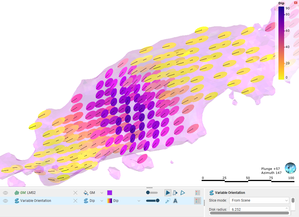
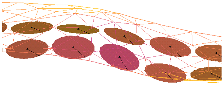
The principal direction of mineralisation can change across a domain, such as when the domain features an undulating, gently-folded structure. Using a single fixed orientation for the sample search and the variogram can result in poor sample selection and weighting locally. Using a variable orientation makes it possible to re-orient the search and variogram according to local characteristics, which results in improved local value estimates. For example, here a variable orientation has been created using a stratigraphic sequence; disks indicate the local search space orientation and are coloured with the dip direction. The output volume of the geological model is shown for context.
Variable orientations can have multiple inputs, including veins, the contact surfaces in a stratigraphic sequence and any mesh in the project.
A variable orientation can be applied to Kriging and inverse distance estimators. You can make as many variable orientations as you wish for each domained estimation, which allows you to experiment with a wide variety of scenarios.
Variable orientations cannot be used with RBF estimators. To achieve a similar capability for RBF estimators, use a structural trend.
The rest of this topic describes how to create and work with variable orientations. It is divided into:
- Visualisation Options for Variable Orientations
- Creating Variable Orientations
- The Variable Orientation in the Project Tree
- Applying a Variable Orientation
- Exporting Rotations
Visualisation Options for Variable Orientations
Variable orientations can be viewed as disks or lines. The grid used for visualisation can be any block model or sub-blocked model in the project or a custom grid can be specified as part of setting up the variable orientation.
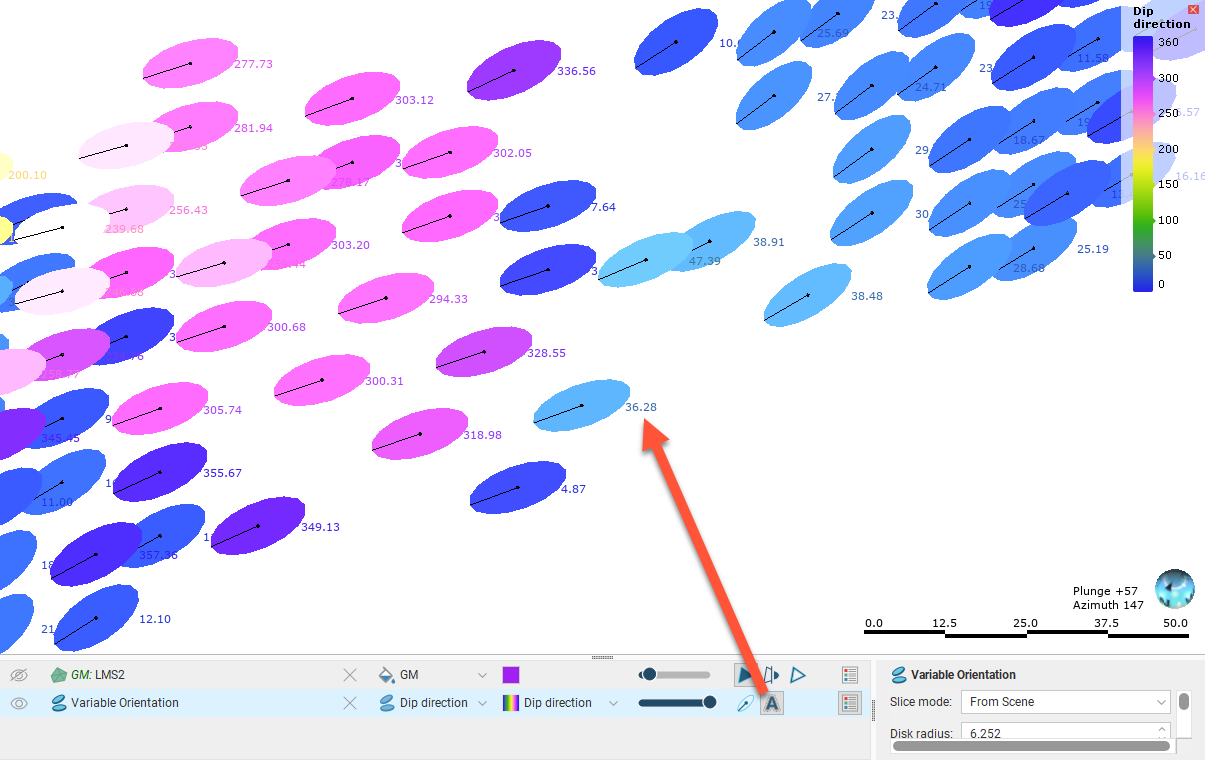
Here a variable orientation is visualised on a custom grid, with disks coloured using the Dip direction values at each point on the grid. Enabling text display (![]() ) shows the values in the scene. The disks are a representation of the local orientation of the maximum-intermediate plane calculated at the chosen centroids. They represent both the search ellipsoid and the variogram, by indicating their principal plane. The line on each disk indicates the position and direction of the major axis.
) shows the values in the scene. The disks are a representation of the local orientation of the maximum-intermediate plane calculated at the chosen centroids. They represent both the search ellipsoid and the variogram, by indicating their principal plane. The line on each disk indicates the position and direction of the major axis.
Search ellipsoids are described using axes of maximum, intermediate and minimum continuity. Variogram ellipsoids are described using major, semi-major and minor axes. Because both the local search ellipsoid and local variogram orientation are indicated by variable orientation disk and line objects in the scene, we will avoid potential confusion by using the terms maximum, intermediate and minimum in this topic, unless specifically discussing variograms.
Click on a disk to view further information about it.
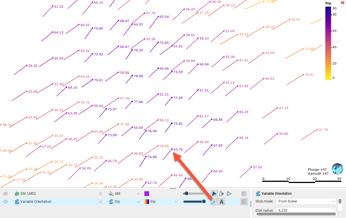
There is also the Show as lines option (![]() ), which hides the disks to reduce visual clutter while still showing the fundamental orientation information in the form of the maximum axis direction for each search space local to each centroid:
), which hides the disks to reduce visual clutter while still showing the fundamental orientation information in the form of the maximum axis direction for each search space local to each centroid:
You can also change the Anisotropy used to display the variable orientation. Options are Isotropic and any variogram models and search spaces defined in the estimation:
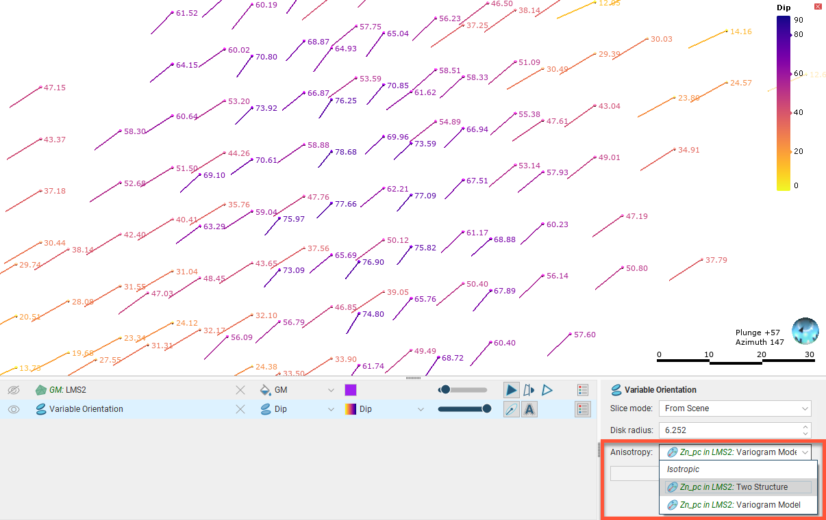
When anisotropy is displayed, the ratio of the maximum-intermediate axis of the chosen object is indicated as a ratio. The actual range is not shown.
Creating Variable Orientations
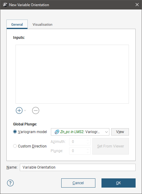
To create a variable orientation, right-click on the domained estimation’s Variable Orientation folder and select New Variable Orientation. Inputs and the Global Plunge are set in the General tab, and how the variable orientation will be displayed is set up in the Visualisation tab.
Selecting the Inputs
Inputs to a variable orientation can include veins, a stratigraphic sequence and any mesh in the project. When a mesh is used, it should be an open mesh that draws out the shape of the undulations of the structure, rather than a closed mesh such as the domain. The facing direction of the surface is relevant; it is used to determine the direction of the surface normal vectors. Each vertex of the mesh is used to generate the orientation, so the resolution of the mesh should be sufficient to capture subtle changes in trend without adversely increasing processing time.
Using closed meshes such as the mesh of the domain used in the estimation is not advised. Doing so may result in boundary effects and inconsistent vector orientations, and the vector may become undefined in the middle of a mesh if components interpolate to zero.
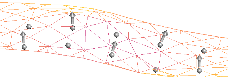
At each vertex of the input mesh, a normal unit vector is calculated from the average orientation of the faces that meet at that vertex. This normal vector is then resolved into three orthogonal component vectors, Δx, Δy and Δz. Take a close look at this slice of an undulating part of a hangingwall mesh shaded according to the face dip:
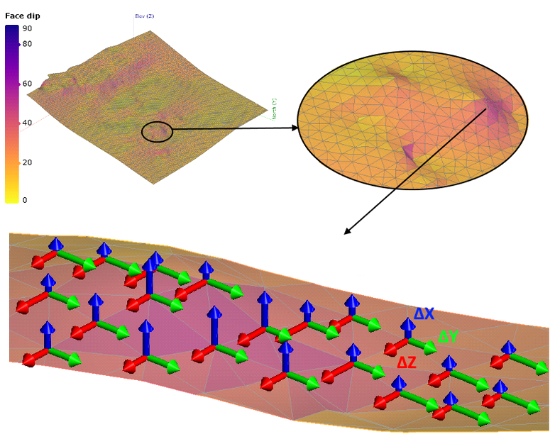
In the above image, the component vectors have been added as explanatory annotations; these are not part of the scene.
Three radial basis functions are then created, one for each of the three orthogonal component vectors. These RBFs use a biharmonic splice basis function of degree zero and ‘reduce’ fit type. Accuracy is set at 1%. These parameters are fixed and cannot be customised or controlled.
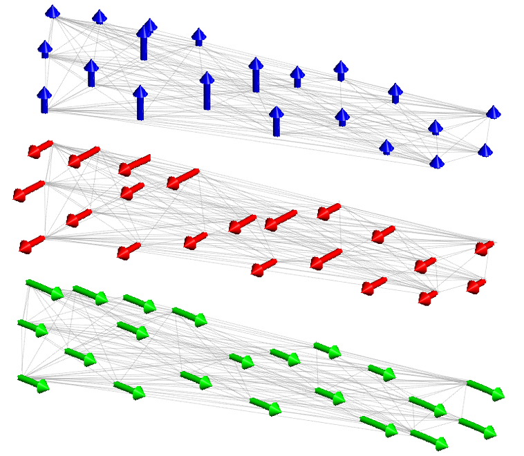
Now that RBFs have been created and we have a continuous function throughout the space of interest, the component vectors for any point in space can be determined, not just at the vertices in the mesh. From the component vectors, the normal vectors can be constructed at any point in space, again, not just at the vertices in the mesh.
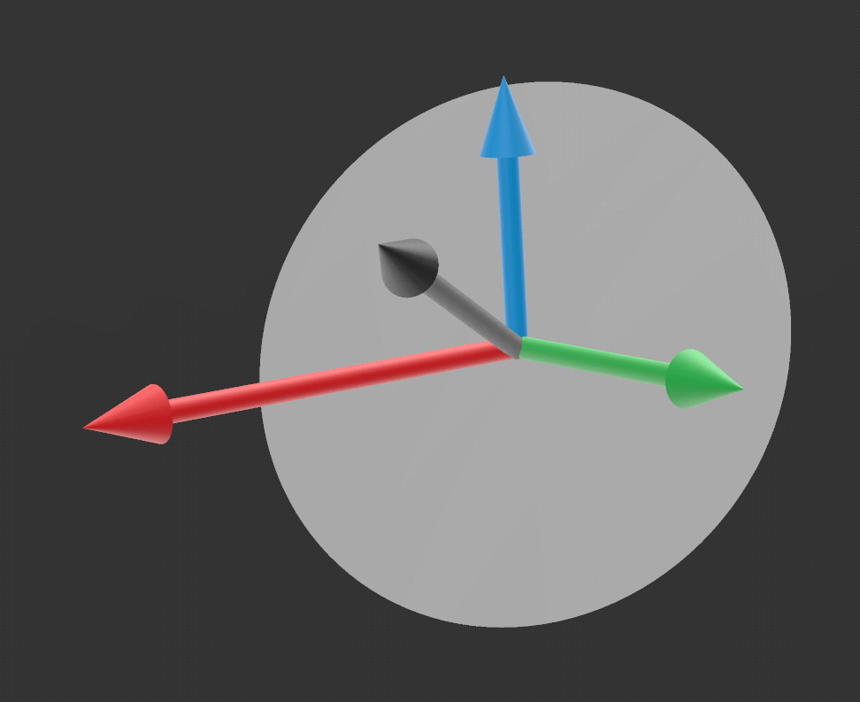
When a normal is reconstructed at any given point in the model, this defines the minimum axis, and, implicitly, the orientation of the principal plane that the maximum and intermediate axes lie on orthogonal to the minimum axis.
Note that although radial basis functions are used in this process to create functions that allow for the determination of normals at any point in space, a variable orientation is not available for use with RBF estimators; it is limited to Kriging and inverse distance estimators. To achieve a similar capability for RBF estimators, use a structural trend.
An important consideration in achieving a reasonable result is inputs that have consistently oriented normals on the mesh used at the start of this process.
- When multiple meshes are used, you need to ensure that the meshes are consistently oriented.
- Veins and stratigraphic sequences are made up of multiple surfaces, and the normals for these surfaces are combined into a single cloud of normal vectors.
- When a vein is used as an input, the hangingwall and footwall surfaces are used. To make normal directions consistent, the hangingwall normals are flipped to point in the same direction as the footwall normals. Common vertices in the footwall and hangingwall, where the vein pinches out, produce duplicate locations with slightly different normals. The two normals at these locations are averaged to give a single normal vector for that location.
- When a stratigraphic sequence is used, each point of each contact surface produces a normal vector.
Closed surfaces have a consistent inside and outside direction. Normals on a closed surface will therefore point either inwards or outwards, resulting in the normals on the opposite side of the mesh pointing in the opposing direction. Interpolating these conflicting normals will lead to sudden unpredictable changes in orientation.
Setting the Global Plunge
Next, the Global Plunge is used to determine the direction of the principal axis on the principal plane. The Global Plunge is a vector defined by either the major axis of the global variogram or globally defined search, or it is set from the view. This vector is used to determine where the direction of the principal axis should lie within the direction of the locally re-oriented principal plane. This is achieved by finding the direction on the local plane that is closest in orientation to the global vector. In practise this amounts to projecting the shadow of the global plunge vector, in the direction of the local normal vector, onto the re-oriented local plane.
You have two choices for the Global Plunge:
- Use one of the variogram models defined for the domained estimation. Select one from the dropdown list.
- Set a Custom Direction. Click and drag in the scene to align the view to the direction of the perceived maximum continuity, then click Set From Viewer. Capture the current scene to bookmark the direction you have set, as the Custom Direction cannot be visualised in the scene.
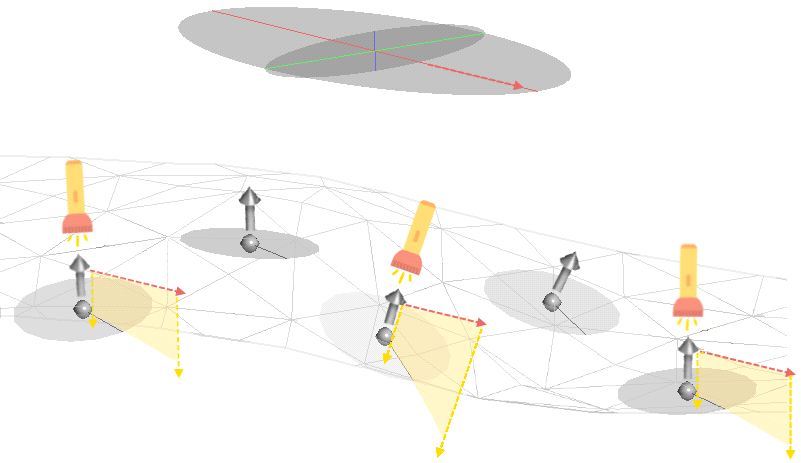
The projected Global Plunge is represented by the black pitch line on each of the variable orientation disks. Visually validate the disk's pitch lines to confirm that the Global Plunge has been applied in the manner you expect.
The Global Plunge is projected onto the principal plane to define the direction of the principal axis. Imagine a flashlight shining down the normal vector towards the principal plane and shining through a variogram model ellipsoid. The shadow cast by the major axis defines the principal direction.
The intermediate axis will lie on the principal plane at 90° to the principal direction axis. Together the normal vector, the principal direction and the intermediate axis orthogonal to them define the orientation for the minimum, maximum and intermediate axes for use at each point required for estimation, reorienting the search and variogram for that specific location in space. These directions are determined for each required location.
When visualised as lines, only the principal direction is shown, pointing away from the reference point. When visualised as disks, a circular disk is added to indicate the principal plane.
If the Custom Direction is left at the default settings of Azimuth = 0 and Plunge = 0, this will be the vector that is projected onto the principal plane. The resulting reorientation of the search space and variogram will likely be inappropriate, particularly for steeply oriented veins. Leapfrog Geo relies upon the expertise of an informed expert to specify a reasonable and valid direction instead of defaulting to a best-guess that may appear meaningful at a cursory glance but may be just as invalid as the more obvious zero values chosen as defaults.
Setting Visualisation Options
In the Visualisation tab, you can choose between visualising the variable orientation on an existing block model or on a custom grid. Here a variable orientation created from a vein is visualised on a block model:
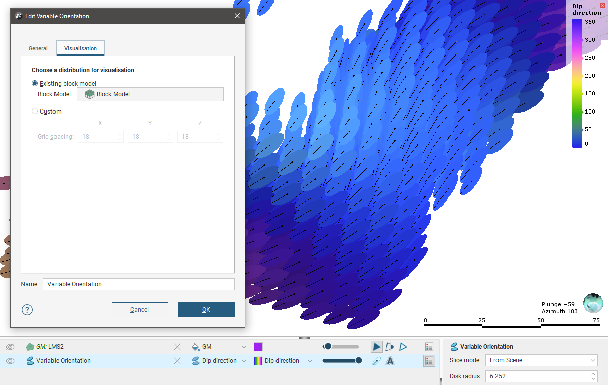
Using a block model or sub-blocked model for visualisation does not evaluate the variable orientation on the selected model. All block models and sub-blocked models in the project can be selected.
Here a variable orientation created from a stratigraphic sequence is visualised on a Custom Grid:
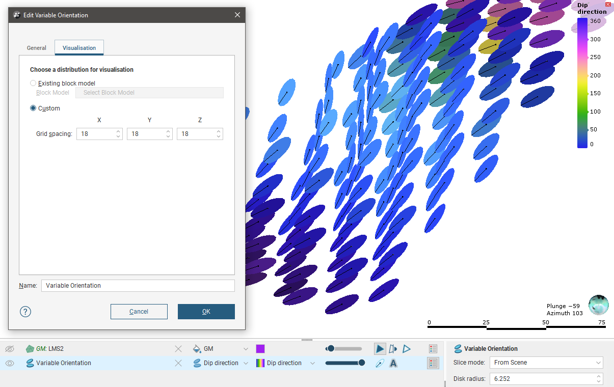
See Visualisation Options for Variable Orientations for more information on displaying the variable orientation.
The Variable Orientation in the Project Tree
Enter a name for the variable orientation and click OK to create it. It will be added to the project tree in the Variable Orientation folder. Expand it to see its parts:
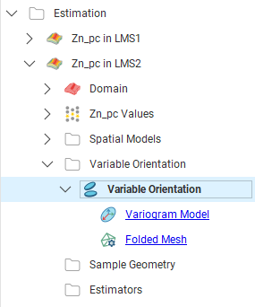
The variable orientation includes links to the variogram model, if used, and to the inputs.
Drag the variable orientation into the scene to check it, and double-click on the variable orientation in the tree to edit it.
You can make multiple copies of a variable orientation, but you cannot copy them to another domained estimation.
Applying a Variable Orientation
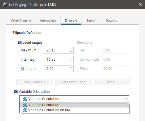
Leapfrog Geo supports variable orientations in Kriging and inverse distance estimators. Double-click on the estimator, then click on its Ellipsoid tab. Tick the box for Variable Orientation and select from those available for the domained estimation:
When a variable orientation is applied to an estimator, the local search can be visualised using the block model interrogation tool.
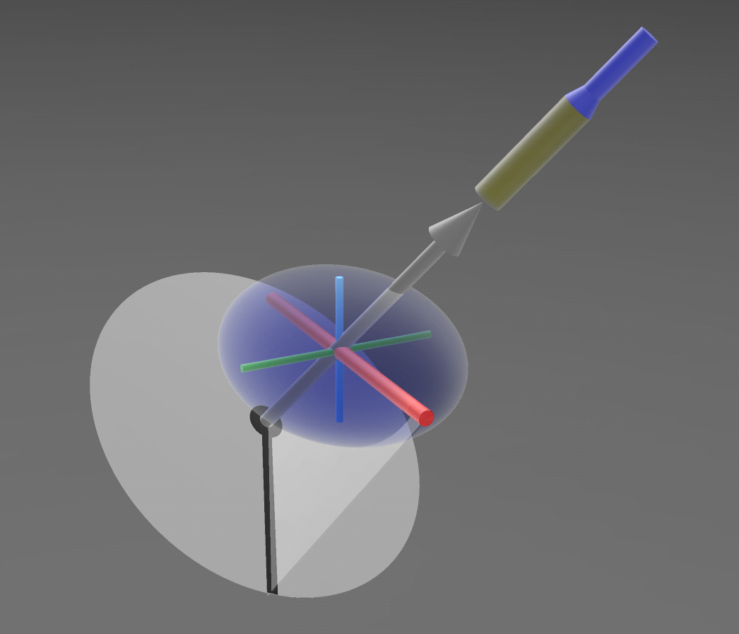
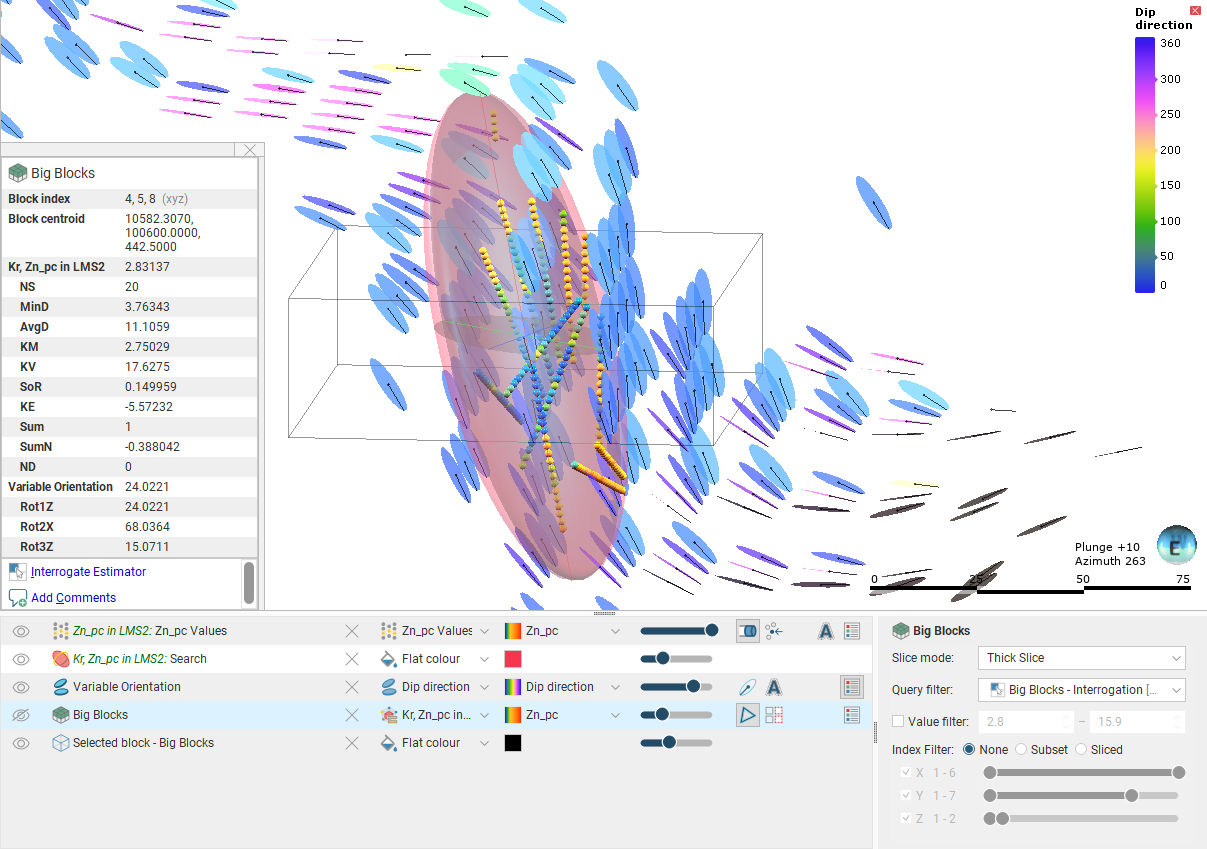
Here one block in a block model is shown with the search area indicated by the ellipsoid widget. The orientation of the ellipsoid reflects the direction set by variable orientation for this block:
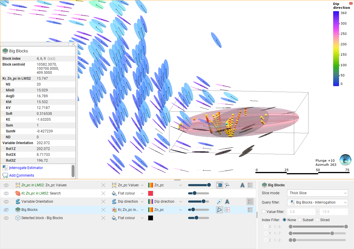
Here the viewing angle is the same but a nearby block is selected, showing a different orientation for the widget. This reflects the effect of the variable orientation on this block, demonstrating that each block can have a different search space and variogram orientation:
See Block Estimate Interrogation for more information on the interrogation tool.
Exporting Rotations
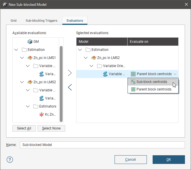
When you evaluate a variable orientation onto a sub-blocked model, you can use the parent block centroids or the sub-block centroids. The default setting is to evaluate onto the parent block centroids:
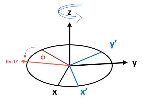
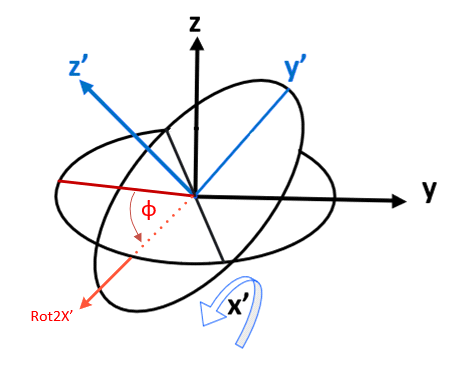
When a variable orientation is evaluated onto a block model or sub-blocked model, the Dip Direction and Dip in the variable orientation are represented in the rotation using the ZXZ convention. Rot1Z is the value of the rotation about the z axis. This turns y into y' and x into x', which is equivalent to the Dip Direction in the variable orientation:
Rot2X is the value of the rotation about the x' axis and is equivalent to Dip:
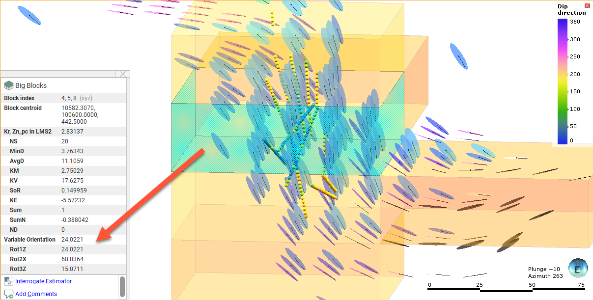
When a variable orientation is evaluated onto a block model or sub-blocked model, you can click on a block to view the rotation information:
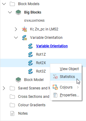
You can right-click on the evaluation in the project tree to view its statistics:
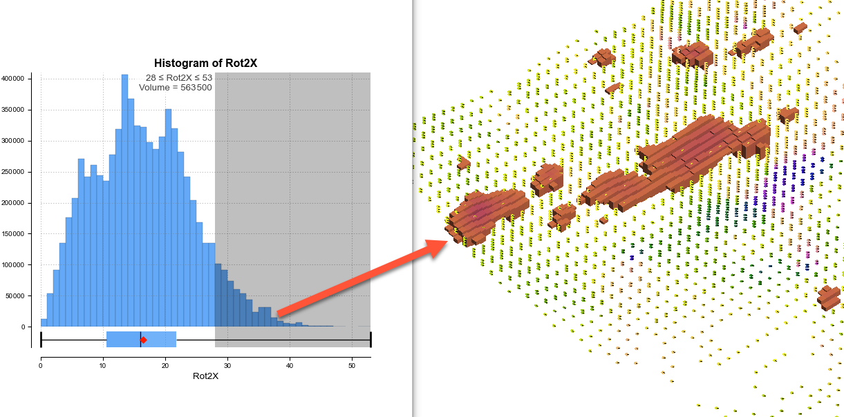
For example, here the histogram is displayed for the Rot2X values. Rot2X varies throughout the surface, indicating that a global trend would not adequately describe the characteristics of surface. The variable orientation is displayed in the scene, along with selected blocks from the block model where the Rot2X values are selected in the histogram. They are highlighted in the scene, indicating the parts of the variable orientation that have the steepest dip:
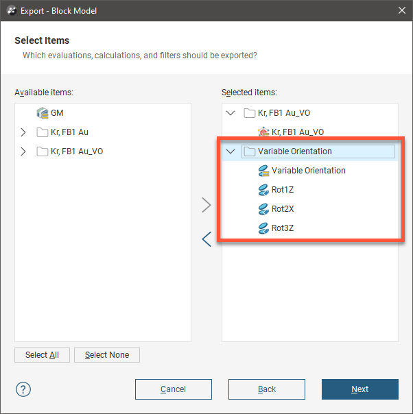
If required, you can export the rotations for use in other packages. When exporting the block model, be sure to select the variable orientation evaluation:
Got a question? Visit the Seequent forums or Seequent support